In this document, we will discuss how to control the order of columns in the SELECT clause in Strategy as well as edit the VLDB parameters to take advantage of the “DISTKEY” distribution style clause on Amazon Redshift.
From the Amazon Redshift Best Practices for Performance community article:
Distribution Key
When using a distribution style of KEY for a table in Redshift, the key value is used to determine the node on which each table row is stored. That is for any table that uses a distribution style of key the rows with the same key value will be distributed to the same node. An important factor in Redshift database design is selecting good distribution keys for fact tables.
The data distribution is defined by using a distribution style of KEY, and defining a distribution key field in the create table DDL. The goal is to have data relatively evenly distributed across the compute nodes for a table, and where feasible, to have tables that join together use the same distribution key. When two tables are joined on their respective distribution keys, matching rows from both tables will reside on the same compute node. In this way, choosing join key as distribution key for related tables that are frequently joined minimizes the need to move data between compute nodes at run time. For star and snowflake schemes the fact table has a different foreign key for each dimension table. Generally, you should choose foreign key of the largest dimension that is frequently joined for your distribution key of your fact table, assuming that this gives relatively even data distribution. If it does not give relatively even distribution, then choose a different distribution key since uneven distribution is more costly to query performance than data movement. Amazon Redshift can perform more efficient joins and aggregations on tables with distribution keys defined rather than using a style of EVEN even if the distribution key is not the column used in the join predicate. You should therefore favor a distribution style of KEY on all dimension tables that don’t use a distribution style of ALL, unless there is no key that will provide even distribution.
For more information on how to choose the best distribution style, please refer to:
https://docs.aws.amazon.com/redshift/latest/dg/c_best-practices-best-dist-key.html
In this scenario, we have a report that generates Multi Pass SQL. We also know we cannot use Derived Tables as our temp table type for this specific report, thus we will need to join the temp tables created during execution to get the final result set.
After reading the “how to choose the best distribution style” article, we know that we can meet the criteria listed in 1-3.
In this example, we have a report that shows “Year”, “Category”, “Region” and two metrics.
The default SQL generated for this report is as follows:
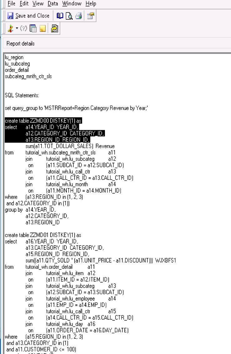
You can see the order of the SELECT clause is Year, Category, Region.
For this example, we have determined that the largest dimension and the highest cardinality attribute is Category, then Year, then Region.
In order to manipulate the order of the SELECT clause, we need to modify the “Attribute weights” of this project. To do this:
1. Go to Project Configuration.
2. Scroll down to Report Defintion -> SQL Generation.
3. Click on Modify in the Attribute Weights section.
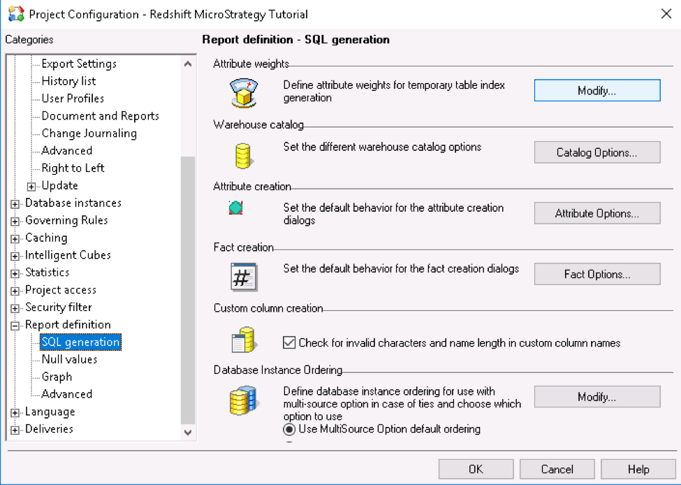
4. Find the attributes you want to “weight” and move them to the right in the order of highest to lowest weight. Where highest will be first.
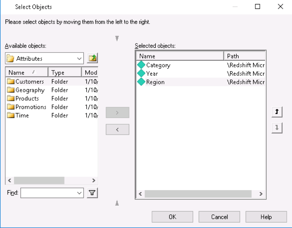
5. Click OK.
6. You will need to purge caches and unload and reload the project (or restart server).
NOTE:
After this change is made, you will see that the order of the SELECT clause has changed and you now see Category, then Year, then Region.
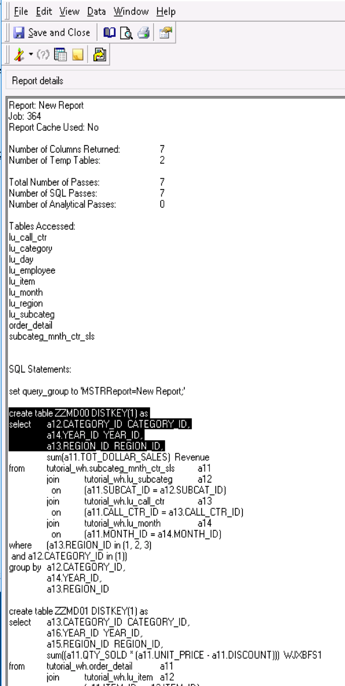
Up to here, we have only manipulated the order of the SELECT clause, but we still need to add the “DISTKEY(1)” clause to the SQL as seen in the examples above and SQL below.
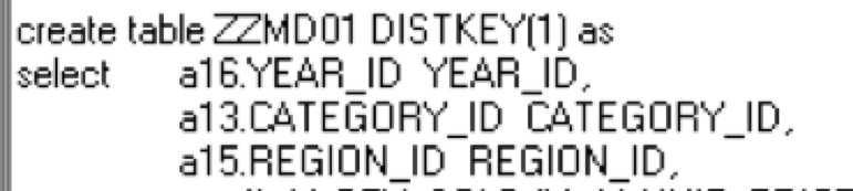
In order to do this, we must edit the DATABASE.PDS file to reposition the “TABLE DESCRIPTOR” VLDB setting to appear before the “as” in the create table statement.
1. Find the DATABASE.PDS file under \Program Files (x86)\Common Files\Strategy on a machine with Strategy Developer.
2. Edit the file with any text editor.
3. Find the section for Redshift by searching for the following:
“<DSSOBJECT TYPE="DBMS" NAME="Amazon Redshift" ID="@dbms156">”
4. Under that section, scroll down to the “VLDB Syntax” PROPERTYSET and find the “Perm Implicit Create Pattern” PROPERTY. You will see the following:
“<PROPERTY NAME="Perm Implicit Create Pattern" VALUE="create table #13 as#6#0#1#2#3#4#5#8"/>”
5. Change the position of the “#8” placeholder to be before the “as” clause. It should now look like this:
“<PROPERTY NAME="Perm Implicit Create Pattern" VALUE="create table #13 #8 as#6#0#1#2#3#4#5"/>
6. Update the DBInstance object.
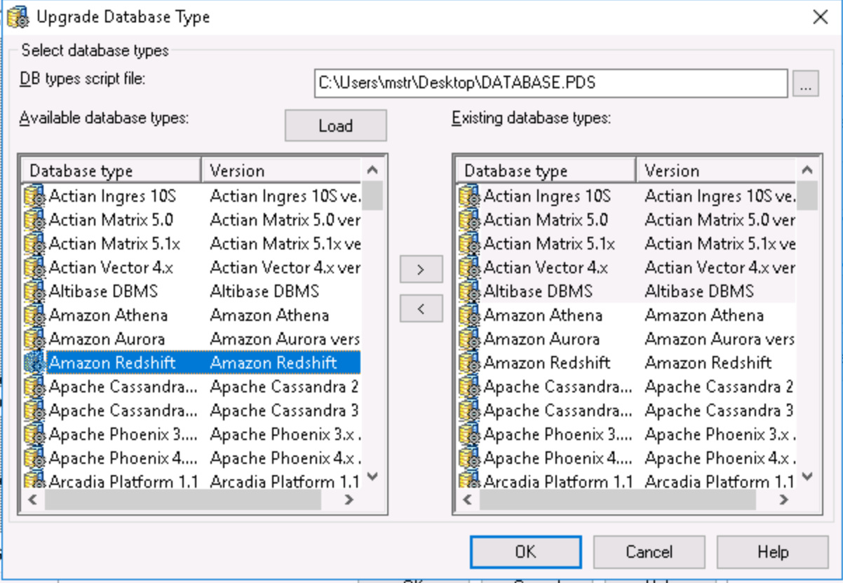
a. Open Strategy Developer, and edit the project DB instance.
b. Click on “Upgrade”.
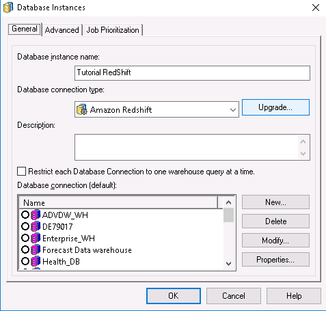
c. Find the modified “DATABASE.PDS” file.
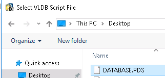
d. Once selected, click on the “Load” button.
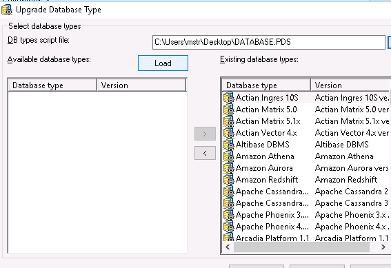
e. Find the “Amazon Redshift” Database type, select it and move it to the right window.
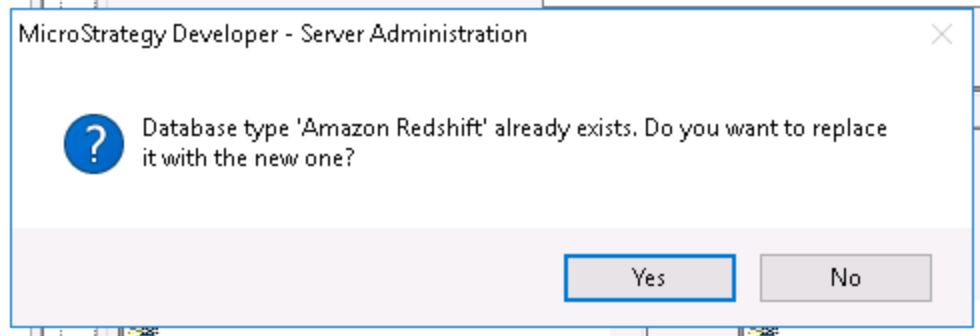
f. Say “Yes” to replacing with the new one.
g. Restart your I-Server.
7. Edit the VLDB properties to add the “Table Descriptor”, "Table Prefix" and change the “Intermediate Table Type" to “Permanent”. This can be done either at the report level or project level.
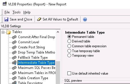
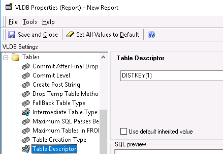
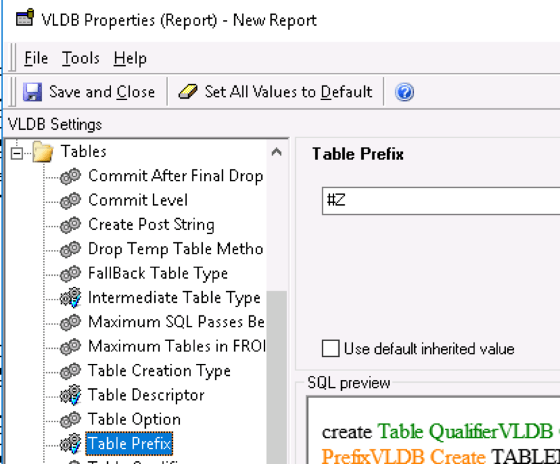
NOTE: True temporary tables in Redshift must be prefixed by “#” and the “Table Descriptor” only applies to “Permanent Tables”, so in order to achieve true temporary table functionality in this scenario, we need to select Permanent tables and then use “#Z” as the table prefix.
8. Once all these steps are done, you can execute your reports to validate the optimized SQL.
create table #ZZZMD00 DISTKEY(1) as
select a12.CATEGORY_ID CATEGORY_ID,
a14.YEAR_ID YEAR_ID,
a13.REGION_ID REGION_ID,
sum(a11.TOT_DOLLAR_SALES) Revenue
from tutorial_wh.subcateg_mnth_ctr_sls a11
join tutorial_wh.lu_subcateg a12
on (a11.SUBCAT_ID = a12.SUBCAT_ID)
join tutorial_wh.lu_call_ctr a13
on (a11.CALL_CTR_ID = a13.CALL_CTR_ID)
join tutorial_wh.lu_month a14
on (a11.MONTH_ID = a14.MONTH_ID)
where (a13.REGION_ID in (1, 2, 3)
and a12.CATEGORY_ID in (1))
group by a12.CATEGORY_ID,
a14.YEAR_ID,
a13.REGION_ID
create table #ZZZMD01 DISTKEY(1) as
select a13.CATEGORY_ID CATEGORY_ID,
a16.YEAR_ID YEAR_ID,
a15.REGION_ID REGION_ID,
sum((a11.QTY_SOLD * (a11.UNIT_PRICE - a11.DISCOUNT))) WJXBFS1
from tutorial_wh.order_detail a11
join tutorial_wh.lu_item a12
on (a11.ITEM_ID = a12.ITEM_ID)
join tutorial_wh.lu_subcateg a13
on (a12.SUBCAT_ID = a13.SUBCAT_ID)
join tutorial_wh.lu_employee a14
on (a11.EMP_ID = a14.EMP_ID)
join tutorial_wh.lu_call_ctr a15
on (a14.CALL_CTR_ID = a15.CALL_CTR_ID)
join tutorial_wh.lu_day a16
on (a11.ORDER_DATE = a16.DAY_DATE)
where (a15.REGION_ID in (1, 2, 3)
and a13.CATEGORY_ID in (1)
and a11.CUSTOMER_ID <= 100)
group by a13.CATEGORY_ID,
a16.YEAR_ID,
a15.REGION_ID
select pa11.CATEGORY_ID CATEGORY_ID,
a13.CATEGORY_DESC CATEGORY_DESC0,
pa11.YEAR_ID YEAR_ID,
pa11.REGION_ID REGION_ID,
a14.REGION_NAME REGION_NAME0,
pa11.Revenue Revenue,
pa12.WJXBFS1 WJXBFS1
from #ZZZMD00 pa11
join #ZZZMD01 pa12
on (pa11.CATEGORY_ID = pa12.CATEGORY_ID and
pa11.REGION_ID = pa12.REGION_ID and
pa11.YEAR_ID = pa12.YEAR_ID)
join tutorial_wh.lu_category a13
on (pa11.CATEGORY_ID = a13.CATEGORY_ID)
join tutorial_wh.lu_region a14
on (pa11.REGION_ID = a14.REGION_ID)
drop table #ZZZMD00
drop table #ZZZMD01
KB439474
